


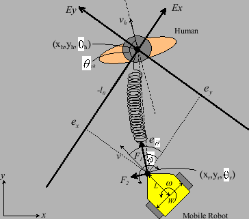
Fig.5 describes the virtual spring model. The world coordinate of the ISpace is converted into a coordinate system whose origin is at the target human.
The direction of a virtual spring at the human side corresponds to the negative direction of the X-axis in the converted coordinate system.
In the following notation, the superscript refers to the coordinate system.
 is the world coordinate of the ISpace, and
  is the coordinate system after conversion.
(1) and (2) represent the state vector of the mobile robot and human in the world coordinate system.
is the coordinate system after conversion.
(1) and (2) represent the state vector of the mobile robot and human in the world coordinate system.
![$\displaystyle ^W{\mbox{\boldmath$x$}}_r=[x_r \: y_r \: \theta_r]^T$](img12.png) |
|
|
(1) |
![$\displaystyle ^W{\mbox{\boldmath$x$}}_h=[x_h \: y_h \: \theta_h]^T$](img13.png) |
|
|
(2) |
 represents the position and direction of the mobile robot,
but it is not on the center of the robot.
It is the world coordinate of the joint, which connects the mobile robot to the virtual spring.
represents the position and direction of the mobile robot,
but it is not on the center of the robot.
It is the world coordinate of the joint, which connects the mobile robot to the virtual spring.  is the length from the mobile robot's center of rotation to the joint.
Both of these coordinates are measured by the ISpace.
The angle between the virtual springs connected to the human and the human's facing direction is expressed as
is the length from the mobile robot's center of rotation to the joint.
Both of these coordinates are measured by the ISpace.
The angle between the virtual springs connected to the human and the human's facing direction is expressed as  .
This parameter is adjustable, and when it is set to
.
This parameter is adjustable, and when it is set to
 , a robot directly follows a human.
The details about will be explained later.
The state vector of the mobile robot in the converted coordinate system is expressed as (3).
, a robot directly follows a human.
The details about will be explained later.
The state vector of the mobile robot in the converted coordinate system is expressed as (3).
![$\displaystyle ^E{\mbox{\boldmath$x$}}_r=[x_e \: y_e \: \theta_e]^T$](img17.png) |
|
|
(3) |
Here, the coordinate system is converted to (4).
![$\displaystyle ^E{\mbox{\boldmath$x$}}_r = {\mbox{\boldmath$F$}}\:
(^W{\mbox{\boldmath$x$}}_r-^W{\mbox{\boldmath$x$}}_h-[0 \; 0 \; \theta_{sh}]^T)$](img18.png) |
|
|
(4) |
Where
 is
is
![$\displaystyle {\mbox{\boldmath$F$}} = \left[
\begin{array}{ccc}
\cos{(\theta_h+...
...heta_{sh})} & \cos{(\theta_h+\theta_{sh})} & 0 \\
0 & 0 & 1
\end{array}\right]$](img20.png) |
|
|
(5) |
The dynamic equations are derived for the case where the elastic power of the virtual spring is applied to the mobile robot, and the input value of the velocity and the angular velocity are determined from the equations.
The state  of the virtual spring is given from the physical relationship between the human and the mobile robot.
It is assumed that the virtual spring transforms ideally and makes a curve which passes along the position
of the virtual spring is given from the physical relationship between the human and the mobile robot.
It is assumed that the virtual spring transforms ideally and makes a curve which passes along the position  of the robot and the origin of the coordinate system.
The deformed length
of the robot and the origin of the coordinate system.
The deformed length  of the virtual spring is approximated as (6).
  is the displacement angle between both ends of the spring, and is represented as (7).
 |
|
|
(6) |
 |
|
|
(7) |
Here, the elastic force which the virtual spring effects on the mobile robot is obtained.
Elastic force  is proportional to
  and acts in the direction of the translational deformation, and
  is proportional to and acts in the direction of bending.
 is the free length of the virtual spring, and represents a set interval between the target human and the mobile robot.
and are as follows:
is the free length of the virtual spring, and represents a set interval between the target human and the mobile robot.
and are as follows:
 |
|
|
(8) |
 |
|
|
(9) |
Here,  and
and  are the virtual spring coefficients of the direction of expansion and bending.
The dimensions of the spring coefficient are
are the virtual spring coefficients of the direction of expansion and bending.
The dimensions of the spring coefficient are ![$[N/m] $](img40.png) and
and
![$ [N{\cdot} rad] $](img41.png) , respectively.
Based on these virtual elastic forces
, respectively.
Based on these virtual elastic forces  , the dynamic equations are derived as follows:
 |
|
|
(10) |
 |
|
|
(11) |
![$\displaystyle \left[
\begin{array}{c}
\dot{v} \\
\dot{\omega} \\
\end{array}\...
...\!F_2\cos{(\theta_e\!-\!\phi)})\displaystyle{\frac{L}{I}}\\
\end{array}\right]$](img45.png) |
|
|
(12) |
 |
|
|
(13) |
 is the mass and
  is the moment of inertia of the mobile robot.
 and
and  are the viscous friction coefficients of translation and rotation, respectively, and each dimension is
 ![$[N{\cdot}s/m]$](img51.png) and
and
![$[N{\cdot} s/rad]$](img52.png) , respectively.
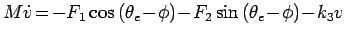
(10) is a dynamic equation about the mobile robot's translational motion.
The left hand side of (10) is the product of the mass and the derivative of the translational velocity.
The first and second terms on the right hand side are the translational factors of and . The third term
is the viscous friction term of both of the forces.
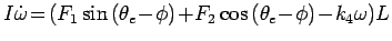
(11) is a dynamic equation about the mobile robot's rotational motion.
The left side of (11) is the product of the moment of inertia and the derivative of the angular velocity.
The first and second term on the right hand side are the rotational factors of and . The third term
is the viscous friction term of the torque.
The torque, which influences the angular velocity, is calculated from the product of and the resultant.
Here,
, respectively.
(10) is a dynamic equation about the mobile robot's translational motion.
The left hand side of (10) is the product of the mass and the derivative of the translational velocity.
The first and second terms on the right hand side are the translational factors of and . The third term
is the viscous friction term of both of the forces.
(11) is a dynamic equation about the mobile robot's rotational motion.
The left side of (11) is the product of the moment of inertia and the derivative of the angular velocity.
The first and second term on the right hand side are the rotational factors of and . The third term
is the viscous friction term of the torque.
The torque, which influences the angular velocity, is calculated from the product of and the resultant.
Here,  and
and  are the translational and angular velocities of the mobile robot.
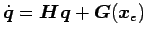
(10) and (11) can be expressed as (12).
The vector and matrix of (12) is replaced with
are the translational and angular velocities of the mobile robot.
(10) and (11) can be expressed as (12).
The vector and matrix of (12) is replaced with
 ,
,
 , and
, and
 of (13).
 and
and  are the velocity of the right and left wheel, respectively, and is the distance between both wheels.
Their relationship is shown in (14).
Based on
are the velocity of the right and left wheel, respectively, and is the distance between both wheels.
Their relationship is shown in (14).
Based on  and
and  from the dynamic equations, and are the input to the mobile robot as actual control input for following the target human.
![$\displaystyle \left[
\begin{array}{c}
V_r \\
V_l \\
\end{array}\right] =
\lef...
... \\
\end{array}\right]
\left[
\begin{array}{c}
v \\
\omega
\end{array}\right]$](img62.png) |
|
|
(14) |
, , and in (10) and (11) are optimised empirically by a simulation based on information about the human; the maximum walking speed, the maximum acceleration, etc.
図 6:
Control block diagram
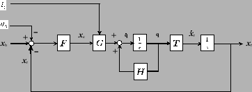 |
The whole of the control system is depicted using a block diagram shown in Fig.6.
Here,  is as follows:
 |
|
|
(15) |
10/06/2005


![$\displaystyle \left[
\begin{array}{cc}
\cos\theta_r & 0 \\
\sin\theta_r & 0 \\
0 & 1
\end{array}\right]$](img66.png)