Fluid Engineering Laboratory |
Fluid Engineering Laboratory |
On the vortical structure in a round jet |
The present research is concerned with the spatial structure in the far-field (or self-preserving) region of an incompressible turbulent round jet. A round free jet has been well investigated both analytically and experimentally , . Although the existence of large-scale structures in this region has been recognized by flow visualization such as LIF (laser-induced fluorescence), there have still been many difficulties in extracting the geometrical detail of the coherent structure due to the temporal and spatial uncertainty of its occurrence.
The organized structure in the far-field region is much less axisymmetric, while that in the near-field region is explained as an apparently axisymmetric mixing layer dominated by vortex rings generated by the Kelvin-Helmholtz instability , . It is supposed that a vortex ring in the near-field grows disturbed as the flow goes downstream and is transformed to a gathering of many pieces of a particular vortex structure, which consists of a pair of radial flows outward and inward with respect to the jet . The scale of these partial structures is comparable to the local width of the jet .
Tso & Hussain measured the velocity field in the far-field region of a round jet by employing an array of several hot-wire probes. They tried to determine the chief spatial modes of the vortex structure from the velocity correlation. They found three major modes—axisymmetric, helical, and double helical—and concluded the helical mode was the most dominant. An LIF visualization by Dimotakis et al.3 also led to a hypothesis that indicated the existence of axisymmetric and helical structures and their transitional structure.
On the contrary, Yoda7 disagreed with the large-scale helical structure and instead suggested a sinusoidal structure from her LIF experiments. The helical structure was also doubted by Ninomiya , who extracted the organized structure by applying LSE (linear stochastic estimation) to the velocity field, which was obtained by three-dimensional PTV (particle tracking velocimetry). A recent numerical study suggests the existence of a group of hairpin-shaped vortices inclined downstream , which might explain the characteristics of the statistical properties reported in earlier research.
Our interest was to learn the actual instantaneous vortex distribution and the organized structure extracted from the velocity field around the jet. Using stereo-PIV, we first measured the velocity fields over the axial cross-section of the far-field region of a round free jet of water at several Reynolds numbers, on the order of 103 based on the nozzle diameter, and visualized a quasi-three-dimensional velocity field, assuming Taylorüfs frozen field hypothesis. Next, we performed a linear stochastic estimation to extract the typical geometrical distribution of the structure.
The flow was a round turbulent water jet emerging from a nozzle (diameter D=5 mm) with Reynolds numbers of 1500 ~ 5000. Water was driven from a reservoir tank out the nozzle at a steady velocity with a top-hat profile into a cylindrical Plexiglas tank (1040-mm high, 780-mm diameter). The water was seeded homogeneously with polyamide-12 tracer particles (Daicel-Degussa, DAIAMID: 1.02 ~ 1.03 sp gr, 40-mm average diameter). The nozzle was placed in the center of the bottom of the cylindrical tank, followed by a section with a flow straightener and a perforated plate below the exit (Fig. 1).
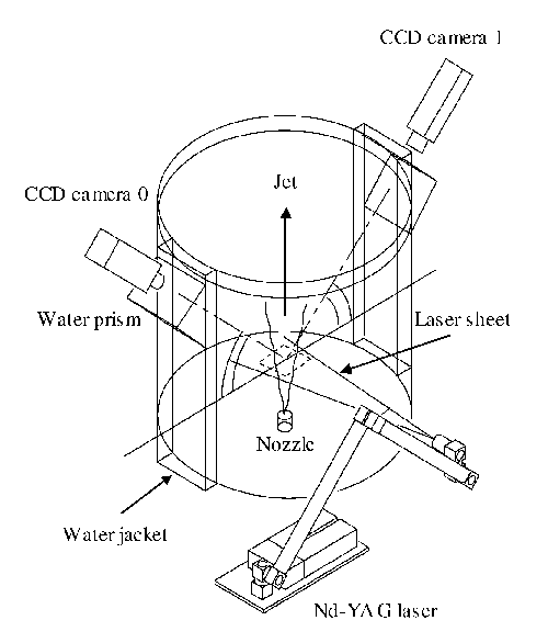
Fig. 1 Schematic of stereo-PIV facility.
We employed a stereoscopic PIV that is capable of resolving time-dependent, three-component velocity in the planes 20D to 50D downstream of the nozzle. These regions of interest were well beyond the minimum far-field criterion4 of ![]() . A laser light sheet of 2 mm in thickness was produced by a Nd-YAG laser (New Wave Research, Minilase-II/30Hz) through a cylindrical lens illuminated planes normal to the streamwise direction, and two CCD cameras (Kodak, Megaplus ES1.0) were positioned to view the tracer particles at the same region of interest in the light sheet plane. The angle between the axes of the two cameras was set to about 90üŗ, and their lenses were mounted to satisfy the Scheimpflug condition. The images captured by the CCD cameras were stored in the host memory of a PC through image grabbers (Imaging Technology, IC/PCI) with a frame rate of 30 fps. Our PIV system could typically capture 450 successive time-dependent pairs of images for both cameras. Since a velocity field could be measured based on the double images, 225 instantaneous three-component velocity maps with 1/15-s intervals were obtained for every run of the experiment.
. A laser light sheet of 2 mm in thickness was produced by a Nd-YAG laser (New Wave Research, Minilase-II/30Hz) through a cylindrical lens illuminated planes normal to the streamwise direction, and two CCD cameras (Kodak, Megaplus ES1.0) were positioned to view the tracer particles at the same region of interest in the light sheet plane. The angle between the axes of the two cameras was set to about 90üŗ, and their lenses were mounted to satisfy the Scheimpflug condition. The images captured by the CCD cameras were stored in the host memory of a PC through image grabbers (Imaging Technology, IC/PCI) with a frame rate of 30 fps. Our PIV system could typically capture 450 successive time-dependent pairs of images for both cameras. Since a velocity field could be measured based on the double images, 225 instantaneous three-component velocity maps with 1/15-s intervals were obtained for every run of the experiment.
The time interval separating the two PIV single exposures was set in order to adjust the mean displacement of the particle at the centerline of the jet to approximately 10 pixels. Since the error in measuring the displacement of the tracers was within 0.2 pixels, the error of the instantaneous velocity was estimated to be 2% of the maximum mean velocity.
The spatial resolution of the velocity measurement was limited by the size of the interrogation spot. Consider a sinusoidal velocity with spatial wavelength L and size N of the interrogation spot of the PIV. Gain G of the measured velocity compared with the true velocity was derived according to the following equation used by Hart11,
![]() .
.
In the present measurements, the dimensions of the interrogation spot were approximately Nz=2.6 mm (28 pixels) in the z direction and Ny=1.9 mm (28 pixels) in the y direction. Thus, the wavelength at which the gain dropped 50% (G=0.5) was computed as 4.3 mm and 3.2 mm in the z and y directions, respectively. This wavelength was approximately 17%-29% of the local jet half-width, and 30-120 times larger than the Kolmogorov scale of the present flow. Obviously, the results shown in this paper will be focused on large-scale structures without resolving small dissipative eddies.
We employed a rectangular Cartesian coordinate system (x, y, z), where x is the vertical (streamwise) distance from the nozzle exit, and y and z are the axes of the plane normal to x. In addition, this coordinate system must be transformed into a three-dimensional polar coordinate system (x, r, q) for subsequent processes. We employed the least squares method on the two-dimensional profile of the streamwise component of the velocity to detect the point where the jet axis penetrates the measurement plane, which was set at the origin, r=0. The mean velocities for the streamwise, radial and azimuthal componentsare U, Vr and Vq, respectively, and u, vr and vq are the velocity fluctuations of each component.
To visualize (or to re-construct) the three-dimensional vortex from the continuous sets of velocity fields obtained, the following assumption was needed. Our stereo-PIV system could resolve the velocity distribution only on a two-dimensional plane; nevertheless, the axis normal to the plane could be locally defined as x* = -Uct if we assumed Taylorüfs frozen field hypothesis, which states that the flow structure remains unchanged as it passes downstream, or, formally, that ![]() for a homogeneous flow. Here Uc is the convective velocity of a spatial structure and U is the local mean velocity. Although a round turbulent jet is not rigorously homogeneous in the x direction, this hypothesis is still valid as long as it is used with a convective velocity of appropriate scale2.
for a homogeneous flow. Here Uc is the convective velocity of a spatial structure and U is the local mean velocity. Although a round turbulent jet is not rigorously homogeneous in the x direction, this hypothesis is still valid as long as it is used with a convective velocity of appropriate scale2.
The distribution of vortices was visualized by employing the swirling strength li, which is a more appropriate index than vorticity, since li represents only the intensity of the rotating fluid motion and does not involve the contribution of shearing transformation12, 13. li corresponds physically to the angular velocity of the local swirling motion and mathematically to the imaginary part of the complex eigenvalue pair of the local velocity gradient tensor. The local velocity field around a particular point at radius r is expressed as
![]() (2.3)
(2.3)
where A is the velocity gradient tensor. Then, we get li as the imaginary part of the eigenvalue l by solving the characteristic equation,
![]() (2.4)
(2.4)
where the constant Q is known to be an index often employed in the identification of vortices. A comparison between the structures visualized by vorticity and li is given in Appendix 1.
The mean and rms velocity profiles are shown in Fig. 2. The radius is normalized by b, which is the local half-value width of U, and the velocities are normalized by Um, which is the maximum value of U. These profiles are obtained by an ensemble average over 450 stereo-PIV realizations for each condition. Most of these statistical quantities show good agreement with previous research, such as Wygnanski and Fiedler2 or Ninomiya9.
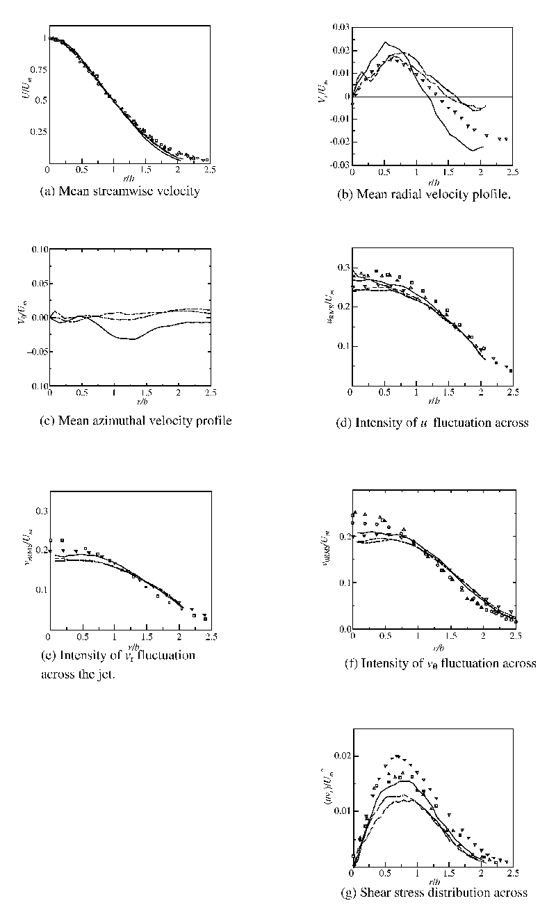
Fig. 2 Statistical quantities of the jet. ü\ü\, Re = 1500 ; ü\źü\, Re = 3000 ; ü\źźü\, Re = 5000 ; üZ, üó, üĀ, - - -, Wygnanski & Fiedler (1969) ; üż, Ninomiya (1992).
The data for the streamwise mean velocity, shown in Fig. 2(a), collapses nicely into the plots of Wygnanski & Fiedler2. The radial velocity in Fig. 2(b) also shows reasonable agreement with Ninomiyaüfs PTV study9, although Vr is fairly low in magnitude, such as 2% of the mean streamwise velocity. The negative values of Vr observed on the outer side of the jet appear to be the entrainment; the flow inward from the surrounding fluid. The mean azimuthal velocity for the Re=3000 and Re=5000 cases, shown in Fig. 2(c), deviates 0.014Um from zero at the maximum, while that for the Re=1500 case shows a slightly larger deviation (0.032Um). The flow in the tank might have some large-scale rotation around the jet axis, although care was taken to ensure the fluid in the tank was quiescent before the experiment. The intensity of the velocity fluctuation in Fig. 2 (d), (e) and (f) also agrees well with previous work.
Figure 2(g) shows the Reynolds shear stress áuvrñ normalized by Um2, where áñ denotes the streamwise average and the ensemble average. The greatest exchange of momentum, which is supposed to involve large-scale vortices, is found to occur at r £ 2b.
Although it is important to estimate the convective velocity of turbulence, Uc, when we assume Taylorüfs frozen field hypothesis to reconstruct an imaginary three-dimensional velocity field, the assumption that Uc is constant for the entire measurement plane across the jet is hardly valid2. The convective velocity in the present jet was measured in the following way. Two-dimensional, two-component velocity maps on the plane including the jet axis were first measured by regular two-component PIV. Then the cross-correlation of the streamwise component of the velocity at two points separated by dx in the streamwise direction and separated by constant time Dt in the temporal direction was calculated. The convective velocity Uc was determined by Uc =dxmax/Dt, wheredxmax is the dx giving the maximum cross-correlation. The profile of measured convective velocity Uc is shown in Fig. 3. The convective velocity is slightly lower than U on the jet axis but increases with radius r to become more than U. The Uc at a higher Reynolds number tends to be lower.
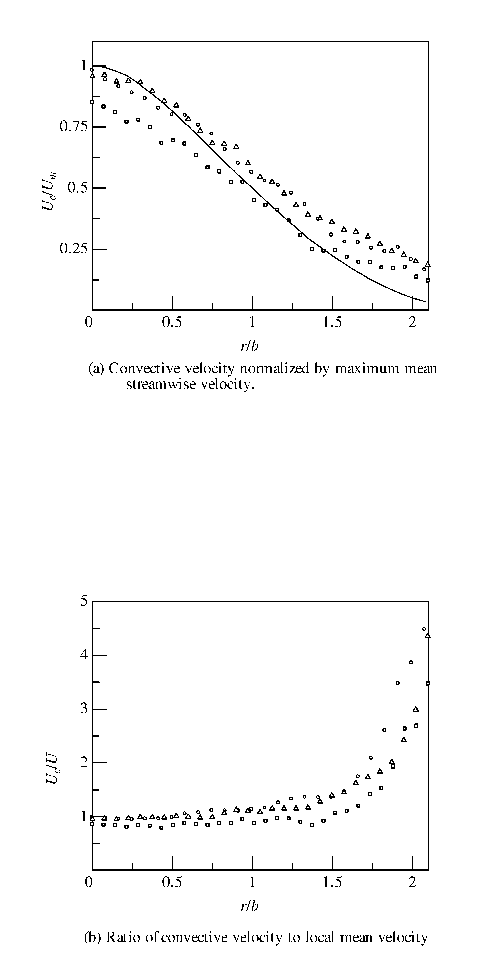
Fig. 3 Convective velocity at x = 30D(a) and ratio of convective velocity to local mean velocity (b). ü\ü\, mean velocity profile at Re = 3000 ; üZ, Re = 1500 ; üó, Re = 3000 ; üĀ, Re = 5000.
Nevertheless, it is still worth using the limited frozen hypothesis to transform temporal quantities to spatial quantities in a range of Dr such that the convective velocity can be considered nearly constant. This statement might sound paradoxical, but it is reasonable as long as we only observe the characteristic organized structure located around a certain radius. In order to ascertain where the large-scale vortices are located on the normal cross-section of the jet, we tentatively tried a li visualization with a certain Uc. Figure 4 shows two examples of the intensity distribution of li with Uc = 0.3Um in a section normal to the jet axis. The shaded gauges on the right side of the diagrams represent the intensity of li using an arbitrary unit of measurement. The white contour indicates the half value of the axial mean velocity U, which has a mean radius of b. Although it still needs to be confirmed whether these diagrams can rigorously be called the spatial distribution of swirling intensity, since the calculation itself is based on the assumption of uniform convective velocity, we can still observe the uneven distribution of li, which forms structures comparable in size to the jet width.
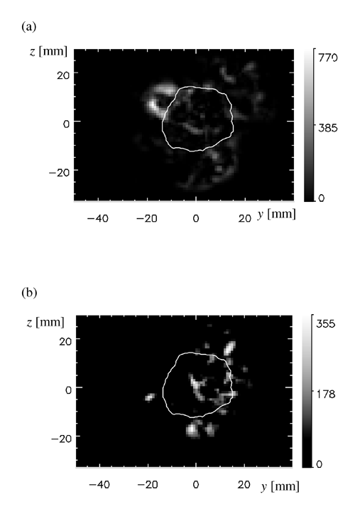
Fig. 4 Intensity distributions of li across the jet at two different instances (a) and (b).
In Fig. 4, some large üglumpsüh of li appear beyond b and near the outer rim of the jet. Near width b, the radial gradient of Uc is significant and causes difficulty in visualizing the structure striding over b without any distortion. On the other hand, near the outer region of the jet, where the gradient of Uc is relatively small, vortex structures could show their reconstructed spatial characteristics, no matter how partially.
Based on the discussion above, we visualized iso-surfaces of li over the imaginary three-dimensional space transformed from the successive time-dependent sets of the two-dimensional velocity fields obtained by stereo-PIV. In this case, the convective velocity Uc was assumed to be Uc =aUm with a constant coefficient a=0.3. The value of the coefficient a (=0.3) is determined empirically (or expediently) in the process of attempting li visualization, but it is also reasonable to represent the convective velocity with r » 1.5b ~ 2.0b, according to the profile of Uc. Note that the effect of the choice of a on the visualized structures is given in Appendix 2.
Figure 5 (a) shows iso-surfaces of li normalized by Um/b at x = 20D, Re = 3000, where the streamwise coordinate (x* coordinate) is defined by the measurement time t as x* = -Uct. At first glance, the hairpin structures, emphasized by the yellow dotted lines, are observed hanging upstream or twining around the entire jet. The li spots found in Fig. 4 are assumed to be cross-sections of these hairpin structures. In order to know the physical size of the hairpin, we traced the vortex strings, which resemble the hairpins empirically (by visual inspection), and measured the width and streamwise distance between successive hairpins. The width, which was defined as the distance between hairpin legs at a relative streamwise location 0.8b downstream from the head of the hairpin, was 0.9b, and the streamwise distance was 1.8b on average, although this value may depend strongly on the method of identification of the hairpin. Note that structures similar to the present hairpin were also observed in the LES studies of the round free jet performed by Suto et al.10 Although it is difficult to abstract a particular structure from the visualization at this moment, we can barely discover helical structures or vortex rings comparable in size to the jet width from any visualization we made. Figure 5(b) shows iso-surfaces of the radial component of velocity, ![]() , together with that of li, where the green and blue surfaces indicate positive and negative values, respectively. It is obvious that li can represent the swirling intensity with the radial flows injecting outward (e.g., label B) through the inside of the hairpin (e.g., label A of Fig.5(a)) and entrained to the rim of the structures (e.g., label C). As shown in Fig.5(c), such an injecting flow induced by the hairpin vortex transfers the streamwise momentum outward, which indicates iso-surfaces of the instantaneous Reynolds shear stress, uvr. Many of the iso-surfaces of uvr are located inside the hairpin loop (e.g., label D), where the flow induced by the hairpin vortices transfers the high streamwise momentum in the core region of the jet toward the outer region. The probability density function of the direction of the velocity fluctuation vector weighted by the Reynolds stress will be discussed in Section 5.
, together with that of li, where the green and blue surfaces indicate positive and negative values, respectively. It is obvious that li can represent the swirling intensity with the radial flows injecting outward (e.g., label B) through the inside of the hairpin (e.g., label A of Fig.5(a)) and entrained to the rim of the structures (e.g., label C). As shown in Fig.5(c), such an injecting flow induced by the hairpin vortex transfers the streamwise momentum outward, which indicates iso-surfaces of the instantaneous Reynolds shear stress, uvr. Many of the iso-surfaces of uvr are located inside the hairpin loop (e.g., label D), where the flow induced by the hairpin vortices transfers the high streamwise momentum in the core region of the jet toward the outer region. The probability density function of the direction of the velocity fluctuation vector weighted by the Reynolds stress will be discussed in Section 5.
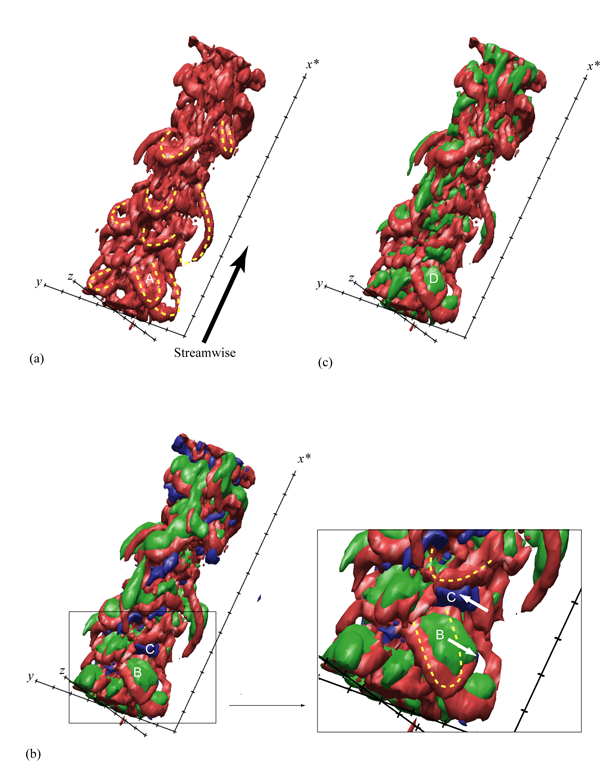
Fig. 5 Vortex strings and their involved flow at x = 20D, Re = 3000, displayed as iso-surfaces of li=0.6b/Um. The tick interval of the x*, y, and z axes is b. The yellow dotted lines on (a) indicate the appearance of vortex strings. (b) is overlayed with the iso-surface of ![]() =0.1Um (green) and
=0.1Um (green) and ![]() =–0.1Um (blue), and (b) also shows a close-up of the hairpin vortex. (c) is overlayed with the iso-surface of uvr=0.015Um2.
=–0.1Um (blue), and (b) also shows a close-up of the hairpin vortex. (c) is overlayed with the iso-surface of uvr=0.015Um2.
Figure 6 shows the visualized iso-surface of li at x = 30D. The scale of the radius is 1.0b. Let us observe the visualizations according to the Reynolds number. The vortices look shrunken at the low Reynolds number (1500) and extended at the high Reynolds number (5000) in the axial direction. This shows that Uc was estimated as larger at the high Reynolds number and smaller at the low Reynolds number. The fall of Uc/Um with the increase in the Reynolds number, which we could also ascertain in Fig. 3, supports this fact. Therefore, it is difficult to impartially discuss the distribution of vortices, but still the visual azimuthal wavelength of the iso-surface doesnüft look very different at any Reynolds number. Note that because the visual azimuthal wavelength (![]() ) is much larger than the spatial resolution (<0.29b) mentioned previously, the observation is not limited by the spatial resolution of the measurement. A more objective measure of the size of the hairpin vortices will be discussed in the next section.
) is much larger than the spatial resolution (<0.29b) mentioned previously, the observation is not limited by the spatial resolution of the measurement. A more objective measure of the size of the hairpin vortices will be discussed in the next section.
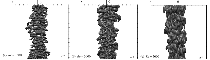
Fig. 6 Iso-surfaces of li at Re = 1500, 3000, 5000, x = 30D. The tick interval is b.
Figure 7 shows vortices from the viewpoint on the jet axis at x = 30D, Re = 3000. Here, the center of curvature of the head of hairpin is found to appear roughly at r = 1.5b, and the azimuthal range of the angle occupied by a hairpin leg seems less than 90üŗ.
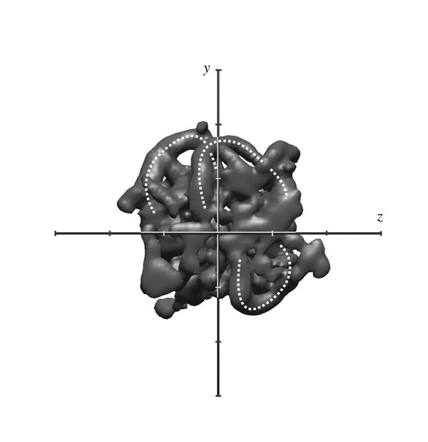
Fig. 7 Vortex strings from the viewpoint on the jet axis, displayed as iso-surfaces of li at x = 30D, Re = 3000. White dotted lines indicate the appearance of vortex strings. The tick interval is b.
In order to extract the geometrical characteristics of the vortex structure more objectively, we applied linear stochastic estimation14 to the velocity field. The quantity of interest is the linear estimate of the conditional average of the velocity field based on an event consisting of the velocity at a single point. The conditional average of the i-th component of the velocity vector at position ![]() based on the j-th component of the event velocity vector at reference position x is written as
based on the j-th component of the event velocity vector at reference position x is written as ![]() . The equations for linear stochastic estimations of the i-th component of
. The equations for linear stochastic estimations of the i-th component of ![]() are
are
![]() .
.
The manipulation for minimizing the mean square error of the estimate leads to linear algebraic equations for the estimation coefficients Lij :
![]()
Once Lij is obtained, the flow field ![]() , called ügconditional eddies,üh14 is given by the event vector. In the present study, the event vector corresponding to the value that contributes the largest amount of the mean Reynolds shear stress was chosen, as previously performed by Ninomiya9. A joint probability function of the angle of the velocity fluctuation vectors weighted by
, called ügconditional eddies,üh14 is given by the event vector. In the present study, the event vector corresponding to the value that contributes the largest amount of the mean Reynolds shear stress was chosen, as previously performed by Ninomiya9. A joint probability function of the angle of the velocity fluctuation vectors weighted by ![]() , referred to as WPDF, measured at all possible azimuthal locations centered at (x,r)=(30D, 1.0b) is shown in Fig. 9. Here, the angles of the vectors are defined as
, referred to as WPDF, measured at all possible azimuthal locations centered at (x,r)=(30D, 1.0b) is shown in Fig. 9. Here, the angles of the vectors are defined as
![]() and
and ![]() ,
,
which are illustrated in Fig. 8 in conjunction with a rotating rectangular coordinate (xüf,yüf,züf). The Reynolds number for this case was Re=3000. There are two distinct peaks at (f,y)=(-0.48 p, -0.18p) and (0.50 p, 0.18p), and each corresponds to inward (vr<0) and outward (vr>0) motions, respectively. Since these peaks represent the fluctuating velocity vector which makes the most contribution to the Reynolds shear stress, we defined the event vector as the unit vector, which has the angle (f,y) where the positive peak is located in the WPDF. Here, only the event vector corresponding to the peak in f>0, which represents outward motion, was used in the following.
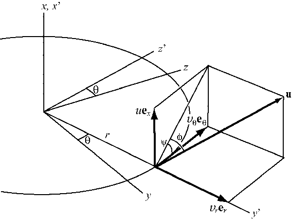
Fig. 8 Definition of angle of velocity vectors, f and y. Unit vectors ex, er and eq are in the xüf, r and q directions, respectively.
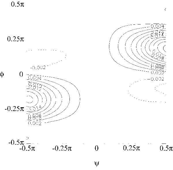
Fig. 9 Joint probability density function of the angle of the velocity fluctuation vectors weighted by ![]() for Re=3000 measured at all possible azimuthal locations centered at (x,r)=(30D, 1.0b).
for Re=3000 measured at all possible azimuthal locations centered at (x,r)=(30D, 1.0b).
The estimated conditional velocity vectors and iso-surfaces of lib = 1.1 at x=30D, Re=3000 are shown in Fig. 10. Here, results for three different reference points are indicated, and a thick arrow represents the event vector. The surfaces for the reference point at yüf=0.7b, where the mean Reynolds stress reaches a maximum, exhibit a C-shaped vortex inclined with respect to the yüf axis, as shown in Fig. 10(a). While the region inside the reference point (yüf<0.7b) has a thick surface of li extending around the reference point, the li iso-surface outside the reference point (züf=0 and yüf>0.7b) is discontinued. In the case of the reference point yüf=1.0b shown in Fig. 10(b), the surface of li outside the reference point (yüf>1.0b) is connected, but is thinner than the other part, and forms a ring-like shape. Such a structure was also found in the linear stochastic estimation performed by Ninomiya9.
The structure estimated for the reference point at yüf=1.5b, shown in Fig. 10(c), exhibits a more pronounced feature: the inside of the reference point (züf=0 and yüf<1.5b) is completely disconnected and the outside of the reference point (züf=0 and yüf>1.5b) is connected by a thick surface, and forms a U-shaped hairpin-like vortex. Since the reference point (yüf=1.5b) is located at the typical center of curvature of the hairpinüfs head visualized in the previous section, the structure estimated here stochastically supports the existence of the hairpin vortices.
The spacing D of the legs of the hairpin is defined as the distance between the two maximums of li in the xüf-züf plane at yüf=1.0b. The contour map of li in the xüf-züf plane at yüf=1.0b for the reference point yüf=1.5b is shown in Fig. 11. There are two distinct peaks, which correspond to the legs of the hairpin shown in Fig. 10(c). The distance between these peaks, D, was measured for each case and plotted in Fig. 12. For all cases in the range of Re=1500-5000, the D is approximately 0.65b. Note that Nickels and Marusic15 proposed a simple structural model of the round jet, which consists of the hairpin-type vortices arranged to extend the head toward the radial direction and the legs toward the centerline. The azimuthal spacing of their proposed hairpin was approximately 0.51b at the leg and 0.17b at the head.
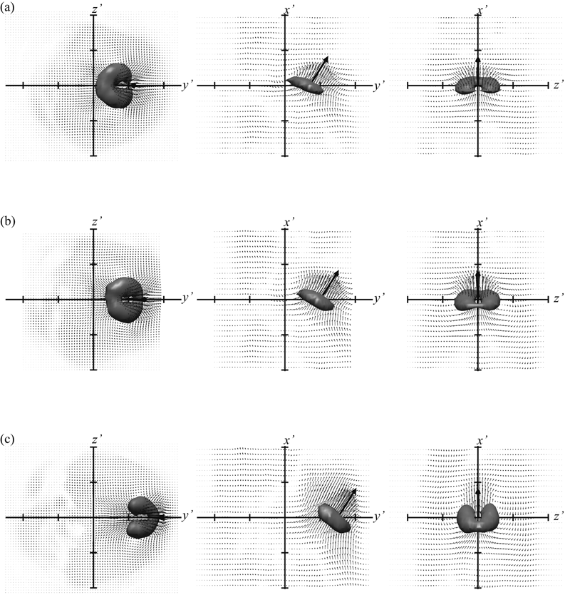
Fig. 10 Estimated conditional velocity vectors and those iso-surfaces of li=1.1b-1 at x=30D, Re=3000. The tick interval is 1.0b.The thick arrows represent the event vector. The reference points are (a) 0.7b, (b) 1.0b and (c) 1.5b, respectively. Three different views for each case are shown from top to bottom.
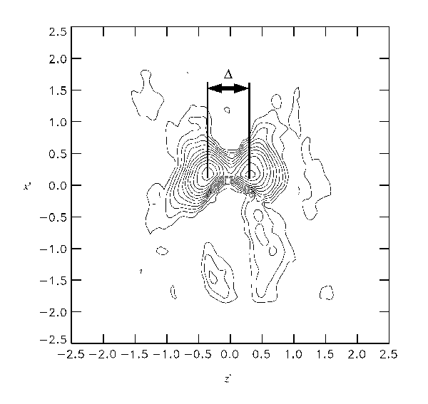
Fig. 11 Contours of li of the estimated conditional velocity vectors in the xüf-züf plane at yüf=1.0b for the reference point yüf=1.5b. The Reynolds number is Re=3000, and the streamwise location where the raw velocity data was taken is x =30D.
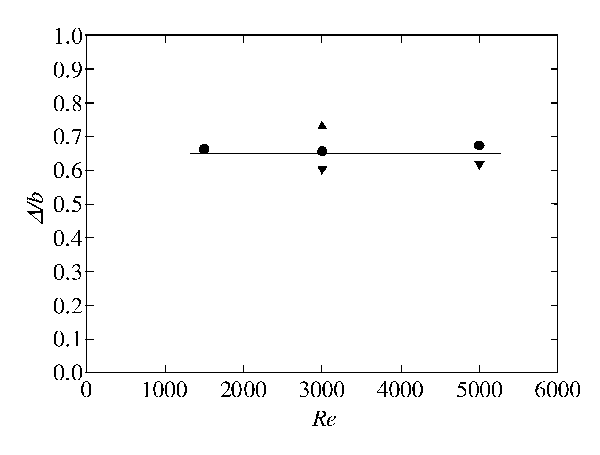
Fig. 12 Spacing D of the legs of the hairpin defined as the distance between two maximums of li in the xüf-züf plane at yüf=1.0b. The reference point was yüf=1.5b.üź, x/D=20; ü£, x/D=30; üŻ, x/D=40.
Stereo-PIV measurement was applied to the self-preserving region of a round free water jet at Re = 1500 ~ 5000. The statistical properties of turbulence obtained in this measurement agreed well with previous analytical and experimental research. Assuming that Uc is locally uniform near the vortex structure around the outer rim of a jet, we reconstructed the quasi-instantaneous three-dimensional velocity field from the successive time-dependent data of three components of the velocity field on the axial cross-section of a jet obtained by stereo-PIV. The vortex structures in the far-field region of the round jet were visualized as iso-surfaces of swirling strength li. Here, groups of hairpin vortex structures were observed in most experimental conditions. The center of curvature of the hairpinüfs head was typically located at r =1.5b.
Linear stochastic estimation revealed a hairpin vortex similar to the one observed in the quasi-instantaneous field. A typical spacing between the legs of the hairpin was 0.65b, which was independent of the Reynolds number in the range of 1500-5000.
For vortex identification, we employed the swirling strength li, which is supposed to be a better indicator than vorticity, since the latter necessarily includes the local shearing transformation of fluid while the former does not. We thought the use of li to be more reliable for a flow such as that of the round jet, which has a thick shear layer, and we were successful in identifying the swirling motion. Figure 13 shows a comparison between the visualizations of vorticity and li. At a glance, both are fairly similar. But, in detail, they are not so similar; for example, in the white dotted circles in Fig. 13, the vortices look warped and sometimes combine when visualized by vorticity.
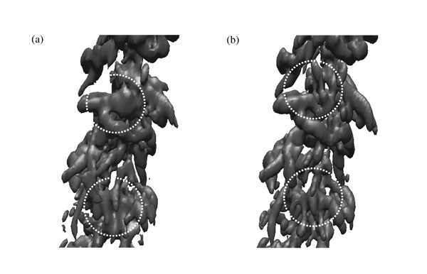
Fig. 13 Visualized vortices, displayed as iso-surfaces of vorticity (a) and li (b) at x = 30D, Re = 3000.
Throughout this paper, the convective velocity Uc was determined to be Uc =aUm with a=0.3. Although the value of a is reasonable in representing the convective velocity of r » 1.5b ~ 2.0b according to the profile of Uc, it is worthwhile to compare the structures visualized using other values of a. Figure 14 shows iso-surfaces of li at x = 20D, Re = 3000, with the same data and viewpoint as that of Fig. 5, except the a for computing the velocity gradient tensor is different. Note that the axial coordinate (x* = -Uct) for displaying iso-surfaces was calculated using a fixed value of a=0.3; otherwise, the structures might be stretched or shrunk by varying the a and comparison would be more difficult. The difference between a=0.2 (a) and a=0.5 (b) is not obvious and both cases show very similar structures, such as the hairpin, as in the case of a=0.3 (shown in Fig. 5(a)). Some heads of the hairpin vortices are slightly larger for a=0.2 than for a=0.5, where the contribution of the streamwise gradient of velocity (e.g., ![]() ) to the li is more significant than for other parts such as the quasi-streamwise hairpin legs, although our conclusion is not affected by this fact.
) to the li is more significant than for other parts such as the quasi-streamwise hairpin legs, although our conclusion is not affected by this fact.
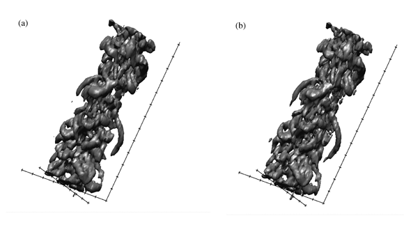
Fig. 14 Visualized vortices, displayed as iso-surfaces of li at x = 20D, Re = 3000 with use of convective velocity Uc = 0.2Um (a) and Uc = 0.5Um (b).
.
I. Wygnanski and H. Fiedler, ügSome measurements in the self-preserving jet,üg J.Fluid Mech., 38, Part 3, 577 (1969).
P. E. Dimotakis, R. C. Miake-Lye, and D. A. Papantoniou, ügStructure and dynamics of round turbulent jets,üg Phys. Fluids, 26, 11, 3185 (1983).
S. C. Crow and F. H. Champagne, ügOrderly structure in jet turbulence,üg J.Fluid Mech., 48, Part 3, 547 (1971).
D. Liepmann and M. Gharib, ügThe role of streamwise vorticity in the near-field entrainment of round jets,üg J.Fluid Mech., 245, 643 (1992).
S. Komori and H. Ueda, ügThe large-scale coherent structure in the intermittent region of the self-preserving round free jet,üg J.Fluid Mech., 152, 337 (1985).
M. Yoda, ügThe instantaneous concentration field in the self-similar region of a high Schmidt number round jet,üg Ph. D. thesis, Stanford University, 1992.
J. Tso and F. Hussain, ügOrganized motions in a fully developed turbulent axisymmetric jet,üg J.Fluid Mech., 203, 425 (1989).
N. Ninomiya, ügThe organized structures in an axisymmetric free jet,üg Ph. D. thesis, Tokyo University, 1992.
H. Suto, K. Matsubara, M. Kobayashi, Y. Hirose, and Y. Matsudaira, ügCoherent Structures of Flow and Scalar Transfer in a Round Jet,üg in Proceedings of the 12th International Heat Transfer Conference (Grenoble, France, 2002), Vol.2, 297.
11 D. P. Hart, ügPIV error correction,üg Exp. Fluids, 29, 13 (2000).
12 M. S. Chong, A. E. Perry and B. J. Cantwell, ügA general classification of three-dimensional flow field, üh Phys. Fluids, 2, 765 (1990).
13 J. Zhou, R. J. Adrian, S. Balachandar, and T. M. Kendall, ügCoherent packets of hairpin vortices in channel flow, üh J.Fluid Mech., 387, 353 (1999).
14 R.J.Adrian, ügStochastic estimation of conditional structure: a review, üh Appl. Sci. Res., 53, 291 (1994).
15 T.B.Nickels, I.Marusic, ügOn the different contributions of coherent structures to the spectra of a turbulent round jet and a turbulent boundary layer, üh J.Fluid Mech., 448, 367 (2001).